
Better understanding IP Routing
Notice: This article is more than 5 years old. It might be outdated.
Today we will look at some of the fundamental principles of IP routing. While these principles and concepts are generic, we will use examples based on AWS networking.
This blog post is not intended to be an all encompassing primer on IP routing. Instead I’ve seen numerous people confused by some of these principles and concepts while either designing networks or troubleshooting them. Therefore it appears to be a good idea to highlight and explain them explicitly.
In a future related blog post we will look at BGP routing in more detail.
Please keep in mind that we will be using AWS VPCs and TGWs to illustrate routing principles. The resulting AWS networking designs are therefore used for illustration purposes and are not suited or recommended for production deployments.
Routing
Routing and more specifically here, IP routing, deals with selecting a path for traffic in an IP network. Routing directs a “hop” within a network on how to forward IP packets based on a routing tables and the destination IP address within the packet.
As we will see later, routing tables maintain information on how to reach various network destinations. Typically they are either configured manually (also known as “Static Routing”) or with the help of a routing protocol (e.g. BGP).
Hop-by-Hop Routing
One of the most fundamental concepts to understand in IP routing is that the actual forwarding decision is made on a hop-by-hop basis. This means that within each hop of the network path, a router makes a forwarding decision based on the local route table. Image this to be like a board game, where at each step in the game it is decided where to go next. Neither the previous nor the next step have any influence on the local decision.
Taking AWS VPCs and Transit Gateways (TGWs) as an example, we can quickly understand how this hop-by-hop decision making plays out, while looking at the routing tables of the VPCs and TGWs (See Figure 1).
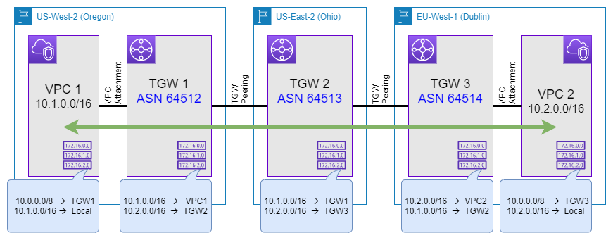
Traffic from an EC2 instance in VPC 1 wanting to reach another EC2 instance in VPC 2 will have to follow this hop-by-hop process through the five routing tables involved here. What do you think? Will traffic from VPC 1 reach VPC 2? Or is there a mistake in the route tables?
Let’s look at each hop, step-by-step:
- VPC 1: Traffic for destinations within VPC 2’s CIDR of 10.2.0.0/16 are send to the TGW 1 over the VPC attachment.
- TGW 1: Inspecting the route table of TGW 1, we can see that traffic for 10.2.0.0/16 is send via a TGW peering to TGW 2.
- TGW 2: Looking at the route table of TGW 2, we can also find an entry for the destination of 10.2.0.0/16. It specifies that traffic should be send via another TGW peering to TGW 3.
- TGW 3: At this point our traffic has already made it into the correct AWS regions. Let’s see what happens next: The route table of TGW 3 indicates that traffic for 10.2.0.0/16 will be forwarded to VPC 2.
- VPC 2: Last but not least, the route table of VPC 2 shows that traffic for the locally used CIDR 10.2.0.0/16 remains within the VPC and is delivered to the corresponding EC2 instance.
But what about the return traffic from VPC 2 to VPC 1? Read on to see how another important principle of IP routing plays a role here.
Directional
Another important principle of IP routing, effectively caused by the hop-by-hop decision making behavior is that path determination is directional. Looking back at the provided example in the previous section (See Figure 1), we only validated that traffic from VPC 1 can reach VPC 2. But we did not validate any information on whether traffic from VPC 2 can reach VPC 1.
I leave it up to you as an exercise to determine if the route tables across the VPCs and TGWs are setup correctly to allow return traffic and thereby enable bidirectional communication. Comment below in case you find a mistake.
When designing route tables or troubleshooting network connectivity it’s always important that you look at traffic flows in both directions and plan or check route table independently for both directions. Also when talking with co-workers, customer, support staff, or anyone alike it is also important that you indicate the direction of the traffic flow that you are referring to.
Asymmetric Routing
What’s even more interesting is that the directional nature of IP forwarding can lead to asymmetric traffic flows. But there is nothing wrong about asymmetric traffic flows and the majority of the Internet relies on it while exchanging traffic between ASNs via Peering or Transit. Think of asymmetric IP traffic flow as a hiking trail loop (See Figure 2). Such hiking trails are often more fascinating than an out-and-return path as you get to see a different set of landscape, plants and animals on the way back as compared to the way out.
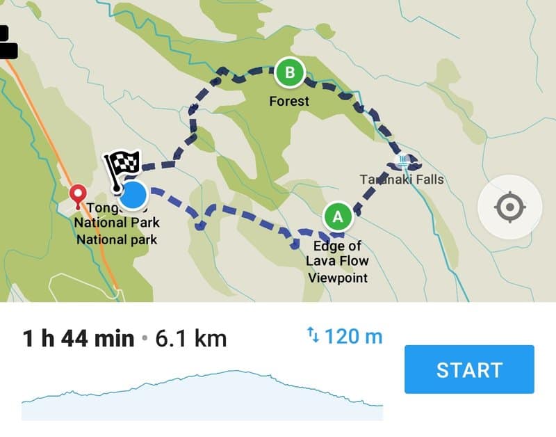
And as long as you make the correct decision at your “routing hops” - aka. a trail fork - you will return to your trail head as well.
Let’s extend the above example using AWS VPCs and TGWs to showcase asymmetric routing. For this we add another TGW and two more TGW peering connections along with changes to the route table (See Figure 3).
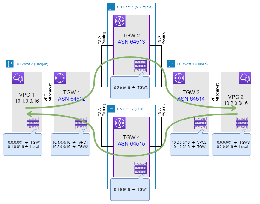
Now, if you follow the path of traffic from VPC 1 to VPC 2, you’ll notice that nothing has changed. Traffic still traverses TGW 1, TGW 2, and TGW 3 on the way to VPC 2. But at the same time look at traffic from VPC 2 to VPC 1. What do you notice? Looking at the route tables of the TGWs you should notice that traffic on the return path from VPC 2 to VPC 1 will traverse TGW 3, TGW 4, and TGW 1, thereby creating and asymmetric path.
This asymmetric traffic flow is depicted with the green arrows.
Route Tables
Next we will look at route tables in a bit more detail. Being able to read and understand route tables, will help you understand the routing decision of the hops within each path.
The most simple route tables have already been depicted in Figure 1 and Figure 3. These routes show a simple mapping between the destination CIDR - also called prefix or network - and the next hop.
Translated into a route table on a Cisco device this might look like this:
CSR1000V-01#sh ip bgp
BGP table version is 297, local router ID is 1.1.1.1
Status codes: s suppressed, d damped, h history, * valid, > best, i - internal,
              r RIB-failure, S Stale, m multipath, b backup-path, f RT-Filter,
              x best-external, a additional-path, c RIB-compressed,
              t secondary path, L long-lived-stale,
Origin codes: i - IGP, e - EGP, ? - incomplete
RPKI validation codes: V valid, I invalid, N Not found

     Network          Next Hop            Metric LocPrf Weight Path
      0.0.0.0          0.0.0.0                                0 i
 *>   10.0.1.0/24      0.0.0.0                  0         32768 i
 *>   10.0.16.0/24     0.0.0.0                  0         32768 i
 *>   10.1.0.0/16      169.254.15.221         100             0 64512 i
Focus on the last line, which effectively translates into: Packets for the prefix “10.1.0.0/16” should be send to the next hop with the IP address of “169.254.15.221”.
Longest prefix match
After this let’s look at longest prefix match, sometimes also referred to as “more specific routing”. This algorithm specifies which entry to be chosen from the IP routing table in case of destination addresses matching more than one entry. For IP routing the most specific of the matching table entries — the one with the longest subnet mask — is called the longest prefix match and is the one chosen.
Consider the below routing table on a Cisco device as an example and especially focus on the last five lines:
CSR1000V-01#sh ip bgp
BGP table version is 297, local router ID is 1.1.1.1
Status codes: s suppressed, d damped, h history, * valid, > best, i - internal,
              r RIB-failure, S Stale, m multipath, b backup-path, f RT-Filter,
              x best-external, a additional-path, c RIB-compressed,
              t secondary path, L long-lived-stale,
Origin codes: i - IGP, e - EGP, ? - incomplete
RPKI validation codes: V valid, I invalid, N Not found

     Network          Next Hop            Metric LocPrf Weight Path
      0.0.0.0          0.0.0.0                                0 i
 *>   10.0.1.0/24      0.0.0.0                  0         32768 i
 *>   10.0.16.0/24     0.0.0.0                  0         32768 i
 *>   10.1.0.0/16      169.254.15.221         100             0 64512 i
 *>   10.1.1.0/24      169.254.16.222         100             0 64513 i
 *>   10.1.2.0/24      169.254.17.223         100             0 64514 i
 *>   10.1.3.0/24      169.254.18.224         100             0 64515 i
 *>   10.1.4.0/24      169.254.19.225         100             0 64516 i
Here we can see that the destination IP address of “10.1.1.1” would match both the entry for “10.1.0.0/16”, as well as the entry for “10.1.1.0/24”. As the entry for “10.1.1.0/24” has a longer subnet mask - it is more specific - and therefore the chosen entry. With that this entry would be chosen and matching traffic send to 169.254.16.222 as the next hop.
Equal Cost Multipath (ECMP)
Usually with IP forwarding there is one egress or outbound path per hop for a given destination IP. This rule can be softened via a routing strategy called Equal-cost multi-path routing (ECMP). With ECMP, packet forwarding to a single destination IP can occur over multiple “best path”.
Again, let’s have a look at an example and consider the below routing table on a Cisco router, especially the last two lines:
CSR1000V#sh ip bgp
BGP table version is 297, local router ID is 1.1.1.1
Status codes: s suppressed, d damped, h history, * valid, > best, i - internal,
              r RIB-failure, S Stale, m multipath, b backup-path, f RT-Filter,
              x best-external, a additional-path, c RIB-compressed,
              t secondary path, L long-lived-stale,
Origin codes: i - IGP, e - EGP, ? - incomplete
RPKI validation codes: V valid, I invalid, N Not found

     Network          Next Hop            Metric LocPrf Weight Path
      0.0.0.0          0.0.0.0                                0 i
 *>   10.0.1.0/24      0.0.0.0                  0         32768 i
 *>   10.0.16.0/24     0.0.0.0                  0         32768 i
 *m   10.0.255.0/24    169.254.13.253         100             0 64512 i
 *>                    169.254.15.221         100             0 64512 i
In this case we can see that we have a multipath route for the destination prefix of “10.0.255.0/24”, where both “169.254.13.253” and “169.254.15.221” are considered as the next best hop. In this case the router device will randomly send out traffic for this destination network over either next hop, while using a 5-tuple hash. A 5-tuple hash refers to a set of five different values that comprise a Transmission Control Protocol/Internet Protocol (TCP/IP) connection. It includes a source IP address/port number, destination IP address/port number and the protocol in use. Here with ECMP and 5-tuple hashing, packets belonging to the same 5-tuple travel to the same next hop, while packets from different 5-tuple may be send to another next hop.
Analogy
IP routing is actually very simple, once you realize that it is similar to hiking without a map:

- You start at the trailhead (source) and want to reach some target (destination).
- Move along the hiking trail to the next fork (router) and look at the signs (route table). Decide which trail (next hop) to chose, in order to reach your destination.
If the sign at the fork lacks an entry to the desired destination, you’re stuck forever and will eventually get eaten by a bear (dropped packet; See Figure 4).
- If you pass the same fork more than once, you’re lost (packet looping) and will eventually run out of food (see below).
- If you pass by more than 64 forks you run out of food, starve and get eaten by a bear (TTL expired).
- If you made it to your desired target (destination), you succeeded. Good job!
- Like IP routing, hiking is bidirectional: You want to get home again, don’t you? Therefore consider the return path as well and follow the above steps.
Summary
In today’s post we took a look at some of the fundamental principles of IP routing. A future post will look in more detail at BGP Routing protocol concepts. Neither of these blog posts is intended to be an all encompassing primer on IP routing or BGP. Instead I’ve seen numerous people confused by some of these principles and concepts while either designing networks or troubleshooting them. Hopefully after reading through this post you feel a bit more confident to design, troubleshoot or just talk about IP networks.
Leave a comment